A Dummy Trading Strategy - II
In this previous post we discussed how you can buy an asset early and cheap, and take incremental profit as it skyrockets. This does not tell you how to buy it (back) at market dip. In this post, we introduce a unified buying-and-selling strategy so that you can make automated trading decisions and make a profit in a volatile market.
The Markov Strategy
We continue with the idea from the previous post:
Whenever the price is multiplied by $p$ since the last action, we sell a number of shares so that an $s$ fraction of shares remains.
where $p \in (1, +\infty)$ and $s \in (0, 1)$ are parameters to tune. We propose a symmetric buying strategy:
Whenever the price is divided by $p$ since the last action, we buy a number of shares so that the number of total shares gets multiplied by $1/s$.
The two strategies can be summarized as:
Whenever the price moves by $p$ since the last action, we move the number of held shares by $s$.
To illustrate this, we show the action table for the first couple of actions (left is selling, right is buying):
| price | $\Delta$ shares | shares | $\Delta$ cash | price | $\Delta$ shares | shares | $\Delta$ cash | |
|---|---|---|---|---|---|---|---|---|
| $p^1$ | $-(1-s) s^1$ | $s^1$ | $+(1-s) (sp)^1$ | $p^{-1}$ | $+(1-s) s^{-1}$ | $s^{-1}$ | $-(1-s) (sp)^{-1}$ | |
| $p^2$ | $-(1-s) s^2$ | $s^2$ | $+(1-s) (sp)^2$ | $p^{-2}$ | $+(1-s) s^{-2}$ | $s^{-2}$ | $-(1-s) (sp)^{-2}$ | |
| $p^3$ | $-(1-s) s^3$ | $s^3$ | $+(1-s) (sp)^3$ | $p^{-3}$ | $+(1-s) s^{-3}$ | $s^{-3}$ | $-(1-s) (sp)^{-3}$ | |
| … | … | … | … | … | … | … | … | |
| $p^k$ | $-(1-s) s^k$ | $s^k$ | $+(1-s) (sp)^k$ | $p^{-k}$ | $+(1-s) s^{-k}$ | $s^{-k}$ | $-(1-s) (sp)^{-k}$ | |
| … | … | … | … | … | … | … | … |
Here, “$\Delta$ shares” means the change in number of held shares, “shares” means new total number of held shares, and “$\Delta$ cash” means the change in cash we hold because of the buying/selling action.
Note that the buys and sells can be interleaved in any arbitrary way, depending on the market. The figure below shows our actions for an asset that rises, drops, and then rises again. (Brackets after the “Buy” or “Sell” means the new number of held shares after the action.)
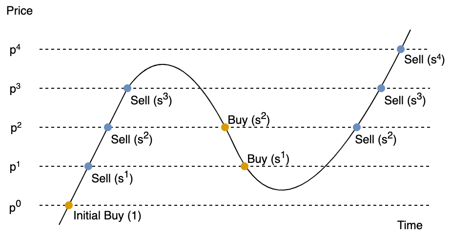
We observe a few nice properties of this strategy:
- We always hold the same number of shares at the same action price. This means our holdings is not amplified nor decayed by market volatility – no matter how the price fluctuates, we will never have to buy more shares we can, or gradually sell all our assets.
- Our cost is bounded, so we don’t need to worry about running out of money and having to abandon the strategy. As long as we keep $s p > 1$, even if the price crashes all the way down, our cash cost $1 + \sum_{j=1}^{k}{(1-s) (sp)^{-j}}$ is bounded by $1 + \frac{1-s}{sp-1}$.
- Our potential revenue is unbounded. Again, as long as we keep $s p > 1$, our cash revenue $\sum_{j=1}^{k}{\frac{1-s}{s} (sp)^j}$ diverges as $k \rightarrow \infty$. As mentioned in the previous post, by choosing $p$ and $s$ appropriately, we can lock up at least half of the market growth (on the log scale).
Since our decision is purely based on the current holdings and the last action point, we call this strategy the Markov strategy.
Bull and Bear
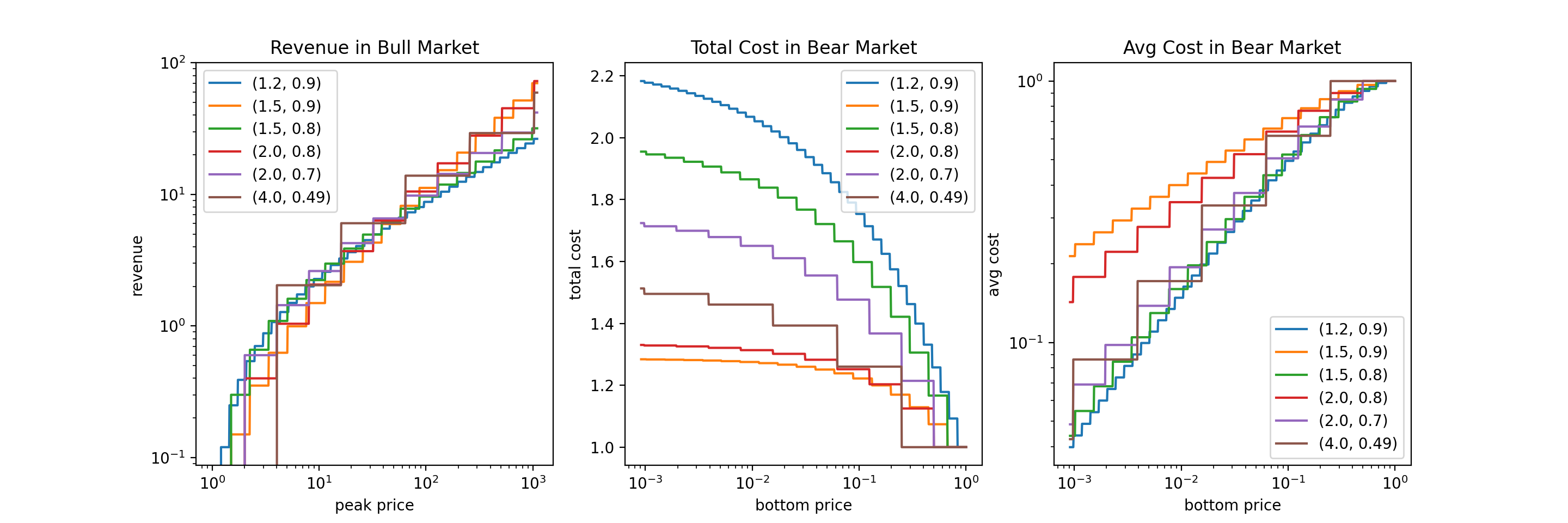
If the market only goes up, we make profit by selling shares gradually, as we discussed before. If the market goes down by a lot (of course we anticipate that it will come back), we “buy the dip” and average down our cost while keeping our total cost capped. The figure below shows the bull market revenue and bear market cost with various values of $p$ and $s$.
Bump and Dip
Now let’s take a look at how the Markov strategy makes money in a volatile market. We show two cases: a market bump and a market dip. The figure below visualizes these two scenarios:
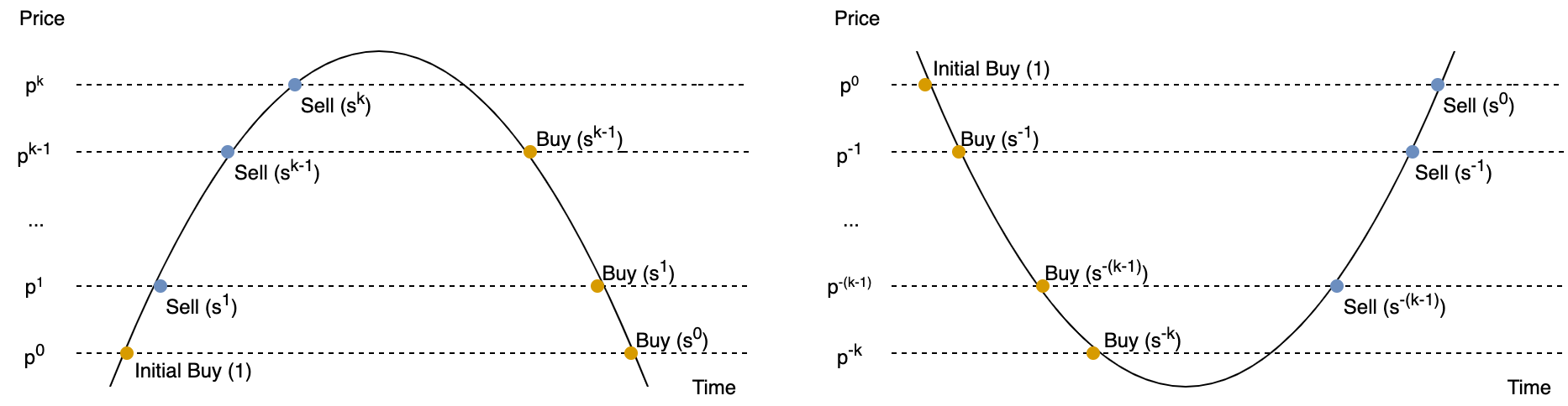
For a bump,
\[Revenue = \sum_{j=1}^{k}{\frac{1-s}{s} (s p)^j} - \sum_{j=0}^{k-1}{(1-s) (s p)^j} = (1-s) (p-1) \frac{(s p)^k - 1}{s p - 1}\]For a dip,
\[Revenue = -\sum_{j=1}^{k}{(1-s) (s p)^{-j}} + \sum_{j=0}^{k-1}{\frac{1-s}{s} (s p)^{-j}} = (1-s) (p-1) \frac{1 - (s p)^{-k}}{s p - 1}\]The figure below shows the revenue for bump and dip with various values of $p$ and $s$.
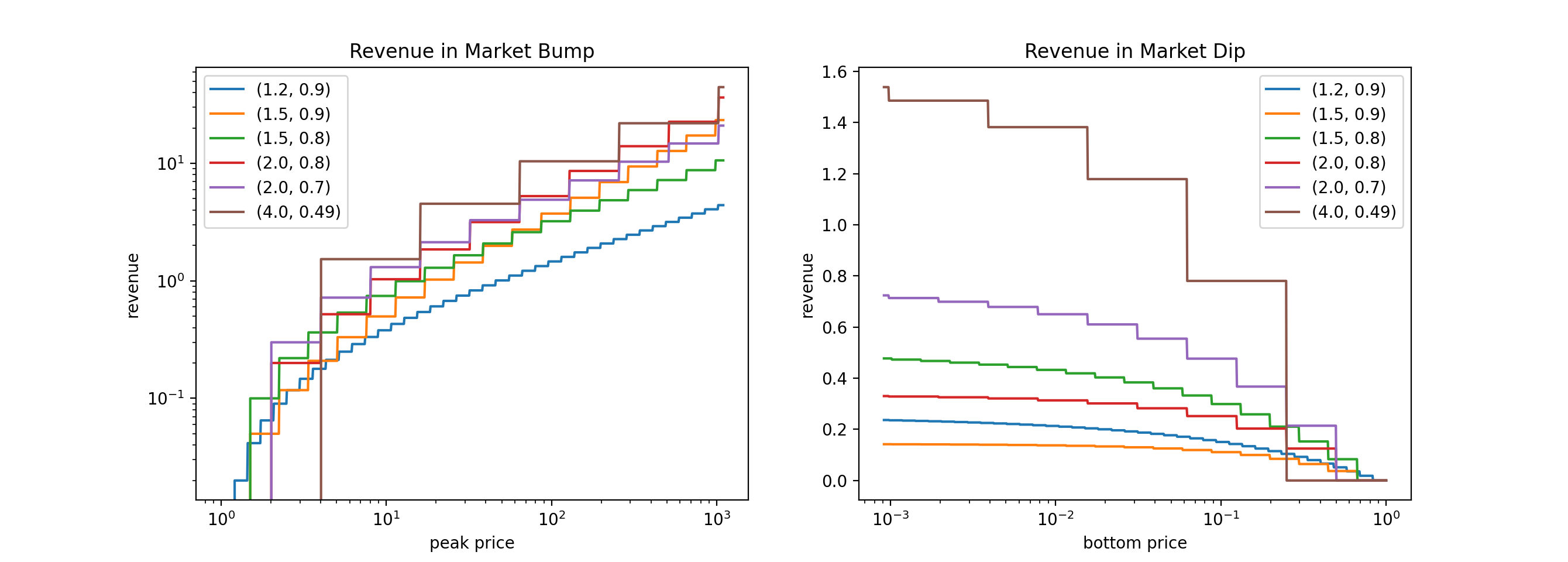
To summarize, the Markov strategy partly takes the ride and partly takes profit during a bull market, buys-the-f***ing-dip during a bear market, and uses the combination of two to make profit during a monkey market.
Backtesting
We backtested our Markov strategy on Bitcoin (BTC) to select parameters $p$ and $s$. First we focus on a monkey market, so we selected daily BTC price data from 02/04/2021 to 05/19/2021. We select a random 3-month window from this range, run the Markov strategy, and compute the mean and std of the final portfolio value.
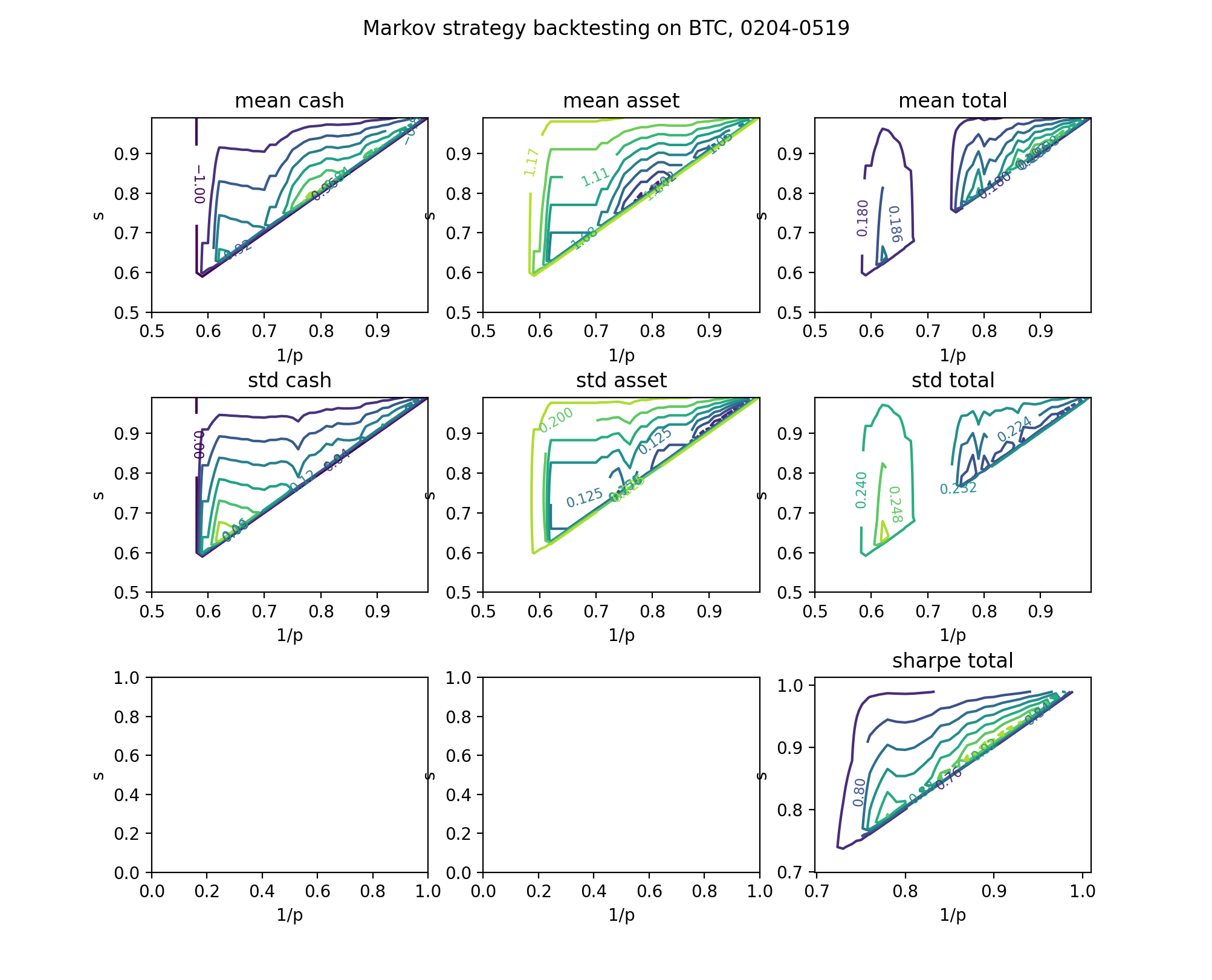
The expected held cash is maximized somewhere where $s p$ is slightly over 1 and $1/p$ is roughly 0.79. However, this parameter setting does not result in a lot of back-and-forth buys and sells in this certain period. I suspect that this revenue mainly comes from coincidence.
On the other hand, the expected total portfolio is maximized somewhere where $s p$ is slightly over 1 and $1/p$ is roughly 0.89. The 3-month sharpe ratio is 1.00, which is pretty good. Looking at the total portfolio graphs, our Markov strategy increases the expected portfolio value while reduces volatility compared to the naive bagholder.
Let’s also take a look at how our strategy will perform in the long term. For BTC, long term is generally bull market. We selected daily BTC price data from a 5-year range (2016 to 2020). We select a random 1-year window from this range, run the Markov strategy, and compute the mean and std of the final portfolio value.
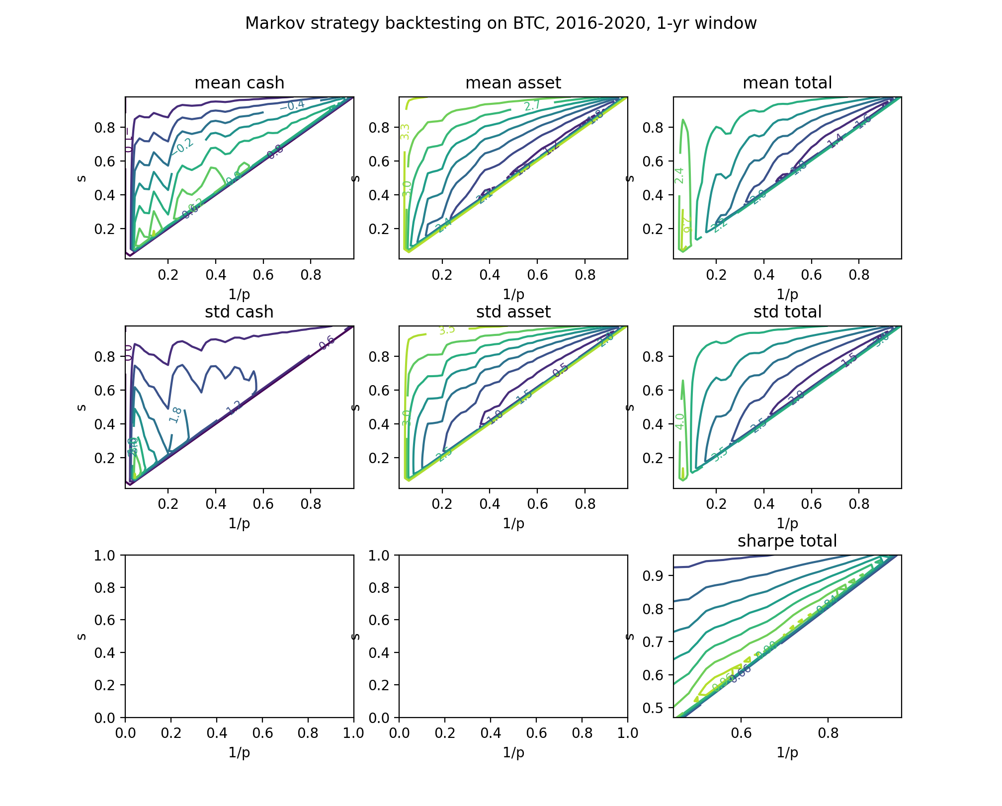
Obviously, long-term horizon favors more patient strategies (i.e. larger $p$). If we keep the same parameter setting as above, we will induce a decrease in total portfolio value compared to the naive bagholder. However, our strategy will still greatly reduce the standard deviation, and yield a much better sharpe ratio.
Therefore, we choose $p = 1/0.89 = 1.1236$ and $s = 0.91$.
Actionable Strategy
My first action was using \$1,000 cash to buy BTC at price \$39,154, and I have 0.025540 shares.
| Buy … shares | If price falls / rises to | Sell … shares |
|---|---|---|
| 0.0030503 | \$27602 | 0.0033520 |
| 0.0027758 | \$31014 | 0.0030503 |
| 0.0025259 | \$34847 | 0.0027758 |
| 0.0022986 | \$39154 | 0.0025259 |
| 0.0020917 | \$43993 | 0.0022986 |
| 0.0019035 | \$49431 | 0.0020917 |
| 0.0017322 | \$55541 | 0.0019035 |
For ETH, I will try to use $p = 2.168$ and $s = 0.618$. My first action was using \$1,000 cash to buy ETH at price \$1681.53, and I have 0.594745 shares.
| Buy … shares | If price falls / rises to | Sell … shares |
|---|---|---|
| 0.367573 | \$642.29 | |
| 0.227172 | \$1681.53 | 0.367573 |
| \$4402.30 | 0.227172 |
More on $p$ and $s$
Let’s take a closer look at the properties of our parameters. We will assume that $sp > 1$.
$r$ and the High-Frequency Limit (HFL)
In a bull market, if price rises to $M$, our revenue is
\[R = \sum_{j=1}^{k}{\frac{1-s}{s} (sp)^j} = \frac{(1-s)p}{sp-1} ((sp)^k - 1)\]where $k = \lfloor \frac{\ln{M}}{\ln{p}} \rfloor$.
Now, consider setting $p$ very close to 1 (i.e. the high-frequency limit (HFL)), so that we won’t need to take the floor: $k = \frac{\ln{M}}{\ln{p}}$. Then we have
\[R = \frac{(1-s)p}{sp-1} (M^{1 + \frac{\ln{s}}{\ln{p}}} - 1)\]This tells us that our revenue growth is $(1 + \frac{\ln{s}}{\ln{p}})$ times the price growth (on the log scale). That is to say, we (asymptotically) capture and realize $(1 + \frac{\ln{s}}{\ln{p}}) \times 100\%$ of the growth. We observe that $\frac{\ln{s}}{\ln{p}}$ is an important factor, and thus we denote $r = -\frac{\ln{s}}{\ln{p}}$. $r \in (0, 1)$ characterizes how our revenue grows as a function of price, at the HFL.
Obviously, we have $s = p^{-r}$. Therefore, at the HFL,
\[R = \frac{(1-s)p}{(sp-1)} (M^{1-r} - 1) \rightarrow \frac{r}{1-r} (M^{1-r} - 1)\]And we (asymptotically) capture $(1-r) \times 100\%$ of the growth. For example, if we set $r = \frac{1}{2}$, our HFL revenue will be $R = \sqrt{M} - 1$, which means we capture roughly half of the growth.
Then we consider a bear market. If price drops to $M$, our total cost is
\[C = 1 + \sum_{j=1}^{k}{(1-s) (sp)^{-j}} = 1 + \frac{1-s}{sp-1} (1 - (sp)^{-k})\]where $k = \lfloor -\frac{\ln{M}}{\ln{p}} \rfloor$. At the HFL, we have
\[C = 1 + \frac{1-s}{sp-1} (1 - M^{1-r}) \rightarrow 1 + \frac{r}{1-r} (1 - M^{1-r}) < 1 + \frac{r}{1-r}\]This means that our possible total cost is capped by $1 + \frac{r}{1-r}$. For example, if we set $r = \frac{1}{2}$, our HFL total cost cap will be 2, which means we will never invest more than twice of what we put in during the first action.
Furthermore, our HFL average cost becomes
\[\bar{C} = \frac{C}{s^{-k}} < \frac{1}{s^{-k}} (1 + \frac{r}{1-r}) = M^r (1 + \frac{r}{1-r})\]which means we (asymptotically) capture $(1-r) \times 100\%$ of the price drop magnitude for averaging down our cost.
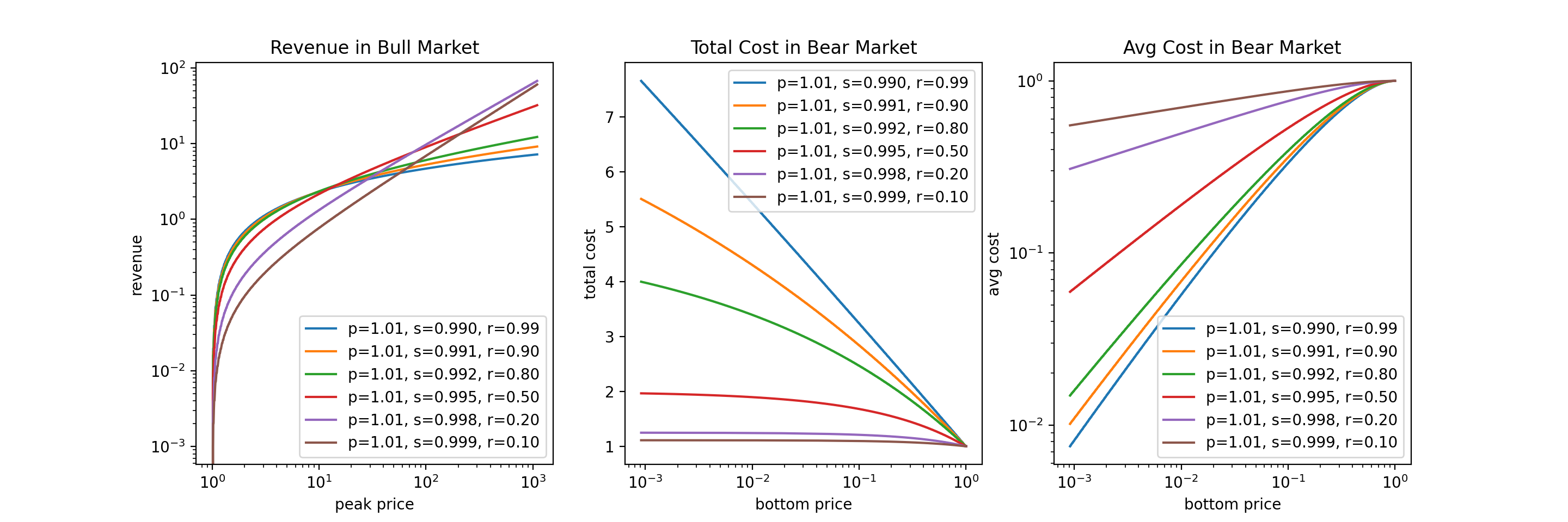
The figure above shows the HFL revenues and costs with varying $r$. We make a few observations:
- In bull market, smaller $r$ performs better if peak price is high; bigger $r$ performs better if peak price is low.
- In bear market, smaller $r$ implies a lower cap of total cost, but is not very effective for averaging down; bigger $r$ implies a higher cap of total cost, but is more effective for averaging down.
Now you might be tempted to say: How about we just pick a super small $r$, like 0.1, which will give us more revenue in s super bullish market, and nicer total cost cap? Well, for one thing, you will need to be very confident that your stock will skyrocket (by that I mean 100x or 1000x), or such choice of $r$ will not give you a margin. For another thing, when moving away from the HFL, smaller $r$ implies higher variance, which we will cover next.
Approximation Error of HFL
In reality we might not be able to reach the HFL, possibly due to rounding errors, non-algo-trading, or transaction fees. Plus, the HFL does not earn us a profit during market bumps/dips. Therefore, we will need to resort to a bigger $p$ and a smaller $s$. We analyze what will happen under a fixed $r$.
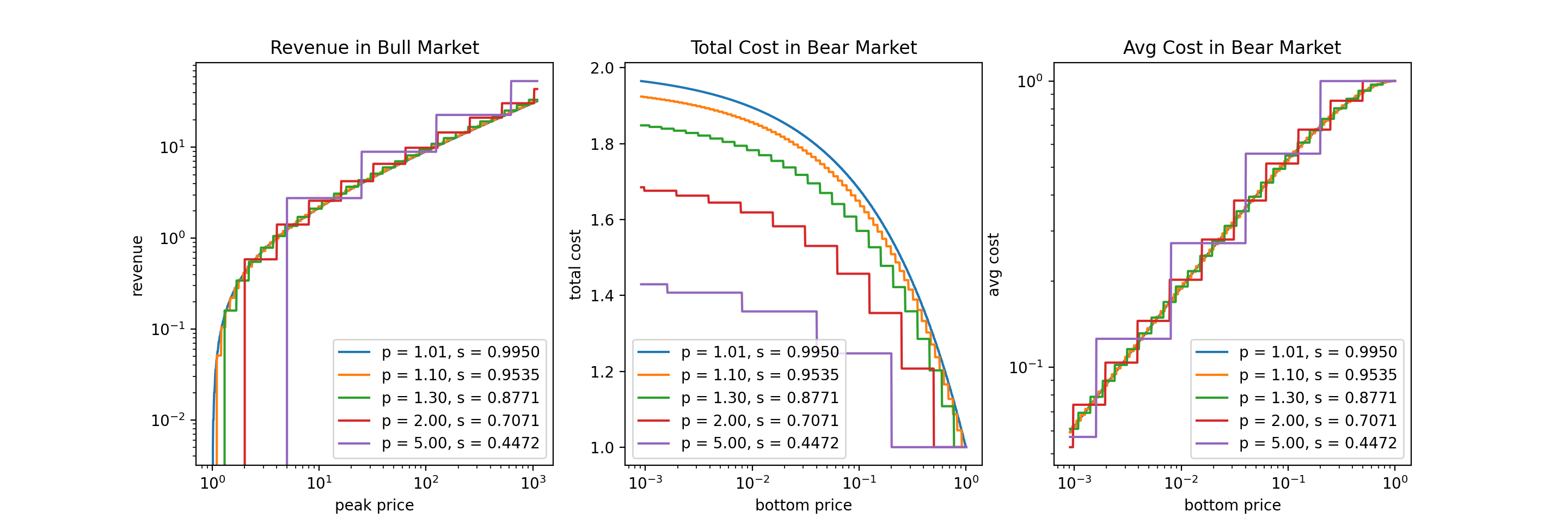
The figure above shows the revenues and costs under $r = \frac{1}{2}$, with varying $p$ and $s$. $p = 1.01$ is a good approximation to the HFL.
We make a few observations:
- As we move away from the HFL, the variance of all metrics (revenue, total cost, average cost) increases.
- In bull market, as we approach the HFL, on average our revenue will decrease, but will converge to the value of HFL.
- In bear market, as we approach the HFL, on average our total cost will increase, but will converge to the value of HFL.
- In bear market, as we approach the HFL, on average our average cost will stay roughly the same, and will converge to the value of HFL.
To summarize, with a given $r$, the choice of $p$ and $s$ is not very consequential. Our primary focus should be choose a good $r$. After that, we can loosely select $p$ and $s$ accordingly which gives a good tradeoff between feasibility and variance.