A Dummy Trading Strategy
There are times in the financial market when a certain asset is traded at a low price but it has huge potential for speculation. Back in 2013 you could buy bitcoins at \$13.50, and by the end of 2017 they were traded at nearly \$20k. When Tesla (TSLA) and Nio (NIO) took off in 2020, their stock prices rallied by 9x and 25x, respectively. In the recent WallStreetBets war with shorting institutions, Gamestop (GME) has had its price skyrocketed because of a short squeeze. The questions is, how can we seize these opportunities and make some profit?
The first trick is to capture the signal and get into the game early, when buying costs are still low. The next problem is when to sell them. No one knows what the peak will be. And to make things worse, when the bubble explodes, the price can drop even faster than it raise, and the asset may become near worthless. Another reason you might want to cash out prematurely is that you want to realize some profit, so that you can maximize expected utility or have something to brag about. A natural way to achieve this is to sell with a designed cadence: when the price rises to this number, sell this amount; when the price rises to that number, sell that amount; and so on.
Now, I will introduce an important pattern of thinking: exponential thinking. It may be tempting to set selling limits with a uniform interval: \$10, \$20, \$30, \$40, … But notice: it is easier to gain \$10 for a \$20 stock than for a \$10 stock; the first one needs only go up by 50%, whereas the latter needs 100%. If you set price limits as an arithmetic sequence like the aforementioned one, you may need to trade more and more frequently, and end up selling more at lower prices. The potential gain is proportional to the current value of the stock, and therefore, by basic calculus, we should think of prices against an exponential curve. That’s why we should set the price limits as a geometric sequence: e.g. \$10, \$20, \$40, \$80, … (More on exponential thinking: Benford’s Law)
Like physicists, we setup the problem as an ideal model. For simplicity, assume that we bought 1 share of stock at price \$1. Trading fractional shares is allowed. The stock will keep rising until it hits \$$M$ per share ($M$ is unknown to us), after which it will become worthless. Our goal is to maximize the revenue.
Here’s our strategy, in formal language. We choose parameters $p > 1, 0 < s < 1$. Whenever the price multiplies by $p$, we sell some shares. The number of shares sold each time is $s$ times the number sold in the previous time.
| When the price rises to … | Sell … shares |
|---|---|
| $p$ | $a_0 s$ |
| $p^2$ | $a_0 s^2$ |
| $p^3$ | $a_0 s^3$ |
| … | … |
| $p^k$ | $a_0 s^k$ |
| … | … |
Apparently we need to make the total number of shares sold add up to 1, which yields $a_0 = \frac{1 - s}{s}$. If the price peaks at $M \in [p^n, p^{n+1})$, our revenue will be
\[R = (1-s) p \frac{(s p)^n - 1}{s p - 1}\]Let’s look at some examples. Let $p = 2$ and $s = 1/2$. At price \$2 we sell 1/2 shares and earn \$1. There we will break even. Then at price \$4 we sell 1/4 shares and earn another \$1. At price \$8 we sell 1/8 shares and earn another \$1. Note that our total revenue is unbounded, but only grows linearly as price rises exponentially.
This time we keep $p = 2$ and let $s = 1/3$. At price \$2 we sell 2/3 shares and earn \$4/3. At price \$4 we sell 2/9 shares and earn \$8/9. Note that we earned less in the second round. Then at price \$8 we sell 2/27 shares and earn \$16/27, which is even less. Our earnings per round is a decreasing geometric sequence, and our total revenue is capped at \$4. This is bad – we capped our gain at 4x, while the stock might rocket to 1000x!
Let’s still keep $p = 2$ and let $s = 2/3$. Things are totally different this time. At price \$2 we sell 1/3 shares and earn \$2/3. At price \$4 we sell 2/9 shares and earn \$8/9. Note that we earned more in the second round! Then at price \$8 we sell 4/27 shares and earn \$32/37, which is even more. Our earnings per round becomes an increasing geometric sequence, and our total revenue is unlimited! Yet the story does not end here – as price rises exponentially, our total revenue also grows exponentially (although still slower than price). Although we started out earning slower (in the first rounds), we unlocked unlimited potential!
To study the root cause of this behavior we go back to the revenue formula. It converges when $p s < 1$, and diverges when $p s > 1$. Our two last examples confirm this. So to make unbounded revenue, you just need to set $p s > 1$, have faith, and have a little bit of patience.
To further analyze the impact of selection of $p$ and $s$, let’s look at the revenues in the following scenarios: $(p = 2, s = 2/3)$, $(p = 4, s = 2/3)$, $(p = 4, s = 1/3)$
| $M$ | $R(p = 2, s = 2/3)$ | $R(p = 4, s = 2/3)$ | $R(p = 4, s = 1/3)$ |
|---|---|---|---|
| [2, 4) | 0.6667 | ||
| [4, 8) | 1.556 | 1.333 | 2.667 |
| [8, 16) | 2.741 | ||
| [16, 32) | 4.321 | 4.889 | 6.222 |
| [32, 64) | 6.428 | ||
| [64, 128) | 9.237 | 14.37 | 10.96 |
| [128, 256) | 12.98 | ||
| [256, 512) | 17.98 | 39.65 | 17.28 |
| [512, 1024) | 24.64 |
Comparing the first two columns tells us what happens when we vary $p$. A lower $p$ yields better revenue at the low multiplier range, while a higher $p$ yields better revenue at the high multiplier range. So if we predict a high $M$, we should use larger $p$. Comparing the last two columns tells us what happens when we vary $s$. A lower $s$ means we sell more aggresively at the beginning, and yields better revenue at the low multiplier range. In contrast, a higher $s$ saves more shares to the long run, and yields better revenue at the high multipler range. So if we predict a high $M$, we should use larger $s$.
If you are looking for a good parameter setting that gives you at least $\sqrt{M}$ revenue, use the golden ratio! Set $p = \phi^2 = 2.618, s = \bar{\phi} = 0.618$. The action table is
| When the price rises to … | Sell … shares | Earn … | Revenue |
|---|---|---|---|
| $\phi^2 = 2.618$ | $\bar{\phi}^2 = 0.3820$ | $\phi^0 = 1.0$ | $\phi^2 - \phi = 1.0$ |
| $\phi^4 = 6.854$ | $\bar{\phi}^3 = 0.2361$ | $\phi^1 = 1.618$ | $\phi^3 - \phi = 2.618$ |
| $\phi^6 = 17.94$ | $\bar{\phi}^4 = 0.1459$ | $\phi^2 = 2.618$ | $\phi^4 - \phi = 5.236$ |
| $\phi^8 = 46.98$ | $\bar{\phi}^5 = 0.09017$ | $\phi^3 = 4.236$ | $\phi^5 - \phi = 9.472$ |
| $\phi^{10} = 123.0$ | $\bar{\phi}^6 = 0.05573$ | $\phi^4 = 6.854$ | $\phi^6 - \phi = 16.33$ |
| … | … | ||
| $\phi^{2k}$ | $\bar{\phi}^{k+1}$ | $\phi^{k-1}$ | $\phi^{k+1} - \phi$ |
| … | … |
What is the optimal strategy?
You may wonder, what is the optimal value for $p$ and $s$? First, we need to define what “optimal” is, i.e. we need to set up a metric. For example, we can choose to optimize for expected revenue, that is, to maximize $\mathbb{E}[R]$.
Then we make a few assumptions. Recall that we denote the peak price as a random variable $M$. The exponential thinking principle means that no matter what the current price is, it is equally likely for it to go further up by a certain percentage. For simplicity we work in the logarithm space. Let $m = \ln{M}$, then the principle translates to $\forall m_0, P(m > k m_0) = c \cdot P(m > m_0)$. This is perfectly captured by the exponential distribution, so we assume that $m \sim \text{exp}(\lambda)$. Here $\lambda$ is a parameter based on the nature of the market.
Now we can compute the probability for each value of the revenue.
| $n$ | $M$ | $m$ | $P_n$ | $R_n$ |
|---|---|---|---|---|
| 0 | $[1, p)$ | $[0, \ln{p})$ | $1 - p^{-\lambda}$ | 0 |
| 1 | $[p, p^2)$ | $[\ln{p}, 2 \ln{p})$ | $p^{-\lambda} - p^{-2 \lambda}$ | $(1-s) p$ |
| 2 | $[p^2, p^3)$ | $[2 \ln{p}, 3 \ln{p})$ | $p^{-2 \lambda} - p^{-3 \lambda}$ | $(1-s) p (1 + sp)$ |
| 3 | $[p^3, p^4)$ | $[3 \ln{p}, 4 \ln{p})$ | $p^{-3 \lambda} - p^{-4 \lambda}$ | $(1-s) p (1 + sp + (sp)^2)$ |
| … | ||||
| $n$ | $[p^n, p^{n+1})$ | $[n \ln{p}, (n+1) \ln{p})$ | $p^{-n \lambda} - p^{-(n+1) \lambda}$ | $(1-s) p \sum_{k=0}^{n-1}{(s p)^k}$ |
| … |
Maximize revenue
Consider setting the metric as the expected revenue, as in the example above. The expected revenue is
\[\mathbb{E}[R] = \sum_{n=1}^{\infty}{P_n R_n} = \sum_{n=1}^{\infty}{\Big[(p^{-n \lambda} - p^{-(n+1) \lambda}) \cdot (1-s) p \sum_{k=0}^{n-1}{(s p)^k}\Big]} \\ = (1-s) p \sum_{n=1}^{\infty}{p^{-n \lambda} (s p)^{n-1}} = \frac{(1-s) p^{-\lambda}}{1 - s p^{-\lambda}}\]when $s p^{-\lambda} < 1$. Otherwise, the sum will not converge, and your expected revenue is infinity! But beware that this is meaningless. As we have shown before, increasing $p$ or $s$ will pump unlikely revenue values, while leaving you a higher probability of winning small (or nothing).
On the other hand, if you stay on the converging side, the gradients
\[\frac{\partial{\mathbb{E}[R]}}{\partial{p}} = -\frac{\lambda (1-s) p^{-(1-\lambda)}}{(p^\lambda - s)^2} < 0 \\ \frac{\partial{\mathbb{E}[R]}}{\partial{s}} = -\frac{p^{\lambda} - 1}{(p^\lambda - s)^2} < 0\]push $p$ and $s$ to the smallest values possible: $p = 1, s = 0$, which means you should sell all immediately after buying (a.k.a. you should not enter the game at all). This is obviously not a desired strategy, but it is the best we get when $s p^{-\lambda} < 1$. Below is a plot for $\mathbb{E}[R]$ under different $p$ and $s$ (with $\lambda = 2.0$):
Maximize utility
The exploding expectation in the previous section implies something wrong with that metric. By the law of diminishing marginal utility, the utility we obtain is not proportional, but sub-linear, to the revenue. Instead of maximizing the expected revenue, we might want to maximize the expected utility. Let’s model the utility with $U = \ln{R}$, and out objective becomes maximizing $\mathbb{E}[\ln{R}]$.
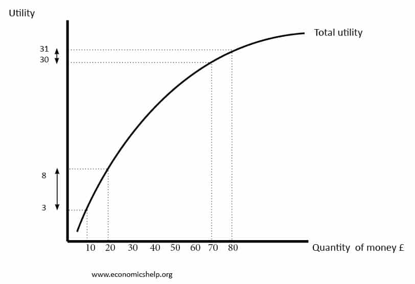
Diminishing marginal utility. Source: Economics Help
The expected utility is
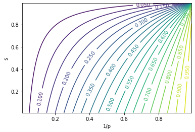
\[\mathbb{E}[U] = \mathbb{E}[\ln{R}] = \sum_{n=1}^{\infty}{P_n \ln{R_n}} = \sum_{n=1}^{\infty}{(p^{-n \lambda} - p^{-(n+1) \lambda}) \cdot \Big[ \ln{(1-s)} + \ln{p} + \ln{\frac{(s p)^n - 1}{s p - 1}} \Big]} \\ = p^{-\lambda} \Big[ \ln{(1-s)} + \ln{p} \Big] + (1 - p^{-\lambda}) \sum_{n=1}^{\infty}{p^{-n \lambda} \ln{\frac{(s p)^n - 1}{s p - 1}}}\]This cannot be solved analytically, so we look at the plot: (with $\lambda = 0.5$)
This indicates a maxima along $s = 0$, so we plug this in, set $\frac{\partial{\mathbb{E}[\ln{R}]}}{\partial{p}} = 0$, and get $p = e^{1 / \lambda}$. This is a beautiful result: we sell off at $M = e^{1 / \lambda}$, i.e. $m = 1 / \lambda$, which is exactly the mean of the exponential distribution.
The shortcoming of this strategy is that you will only have a 37% chance of making any revenue. And that is based on the premise that your estimation of $\lambda$ is accurate. In the other 63% time you will lose everything.
Maximize $\mathbb{E}[\frac{R}{M}]$
Another strategy is to maximize the expectation of $\frac{R}{M}$, that is, portion of growth that we realized. The expectation is computed as follows.
\[P_n \mathbb{E}_n[\frac{1}{M}] = P_n \mathbb{E}_n[e^{-m}] = \int_{n \ln{p}}^{(n+1) \ln{p}}{e^{-m} \cdot \lambda e^{-\lambda m} dm} = \frac{\lambda}{1 + \lambda} p^{-(1 + \lambda) n} (1 - p^{-(1 + \lambda)}) \\ \mathbb{E}[\frac{R}{M}] = \sum_{n=1}^{\infty}{P_n \mathbb{E}_n[\frac{R}{M}]} = \sum_{n=1}^{\infty}{P_n R_n \mathbb{E}_n[\frac{1}{M}]} = \frac{\lambda}{1 + \lambda} (1 - p^{-(1 + \lambda)}) \frac{(1-s) p}{sp - 1} (\frac{s p^{-\lambda}}{1 - s p^{-\lambda}} - \frac{p^{-(1 + \lambda)}}{1 - p^{-(1 + \lambda)}}) \\ \frac{\partial}{\partial{p}} \mathbb{E}[\frac{R}{M}] \propto -\frac{\lambda (1-s) p^{\lambda - 1}}{(p^\lambda - s)^2} < 0 \\ \frac{\partial}{\partial{s}} \mathbb{E}[\frac{R}{M}] \propto -\frac{p^\lambda - 1}{(p^\lambda - s)^2} < 0\]Again, the gradients push $p$ and $s$ to the smallest values possible: $p = 1, s = 0$, and you shouldn’t have played at all!
Penalize for variance
We love profit, but we also hate risk. We want to achieve more stable revenue, so we can add a penalty term to our metric that captures the variance. We denote the standard deviation of the revenue as $\sigma[R]$.
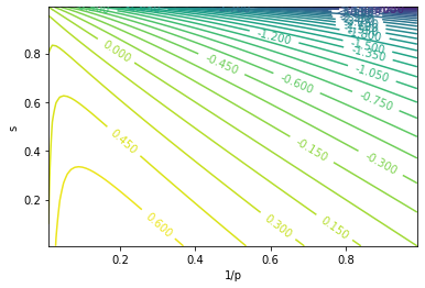
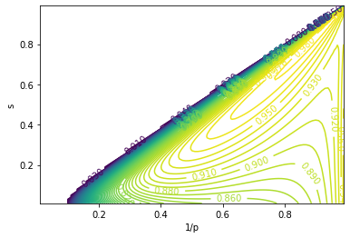
\[\mathbb{E}[R^2] = \sum_{n=1}^{\infty}{P_n R_n^2} = \frac{(1-s)^2 p^{2 (1 - \lambda)} (p^\lambda + s p)}{(1 - s^2 p^{2 - \lambda}) (1 - s p^{1 - \lambda})} \\ \sigma[R] = \sqrt{\mathbb{E}[R^2] - \mathbb{E}[R]^2} = \frac{(1-s) p^{1 - \lambda}}{1 - s p^{1 - \lambda}} \sqrt{\frac{p^\lambda - 1}{1 - s^2 p^{2 - \lambda}}} = \mathbb{E}[R] \sqrt{\frac{p^\lambda - 1}{1 - s^2 p^{2 - \lambda}}}\]From there we can maximize for something like $(\mathbb{E}[R] - \sigma[R])$. Here’s the plot: (with $\lambda = 0.25$)
We see a maxima at $p = 2.5, s = 0.24$. However, this method is not very robust, as the maxima may degenerate with other choices of $\lambda$, and we will be forced to either sell all when it hits a certain price, or to sell a bit whenever the price makes the slightest move. $\lambda = 0.3$ shows the latter case:
Mean-Variance Analysis
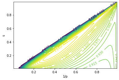
The idea of mean-variance analysis is to achieve the maximum return for a given level of risk (i.e. variance). Equivalently, we want to minimize the standard deviation for a given expected return. We plot $(\sigma[R] / \mathbb{E}[R])^2$: (with $\lambda = 0.5$)
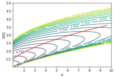
The red line denotes the optimal $p$ for each value of $\mathbb{E}[R]$. We make the following observation:
- For a given expected return, there is always an optimal $p$ that minimizes risk at this return level. The optimal $p$ increases as return level increases.
- With better return level comes the higher risk, which is in line with common beliefs.
Gamma prior
TODO