Defying Transformers: Searching for "Fixed Points" of Pretrained LLMs
Transformers are transformative to AI. Are there things that cannot be transformed by Transformers?
One problem that motivates this quest is the repetition degeneration in LLMs. The seminal 2019 paper by Holtzman et al. revealed this repetition problem and proposed top-$p$ sampling as a mitigation. That said, more recent LLMs are still plagued by repetition, as discussed in the following papers: 1, 2, 3, 4.
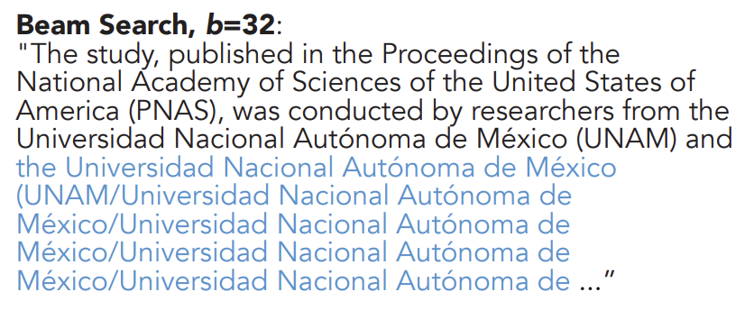
Figure 0: Repetition in text generated by LLMs. Image credit Holtzman et al.
Let’s consider a simplistic setting, where a single input token is repeatedly decoded by a Transformer model. If we view the forward pass of a Transformer as a function $T$ that takes input sequence $[y_1, y_2, …, y_n] = T([x_1, x_2, …, x_n])$, our task is to find an $x$ where $[x, x, …, x] = T([x, x, …, x])$. There’s a mathematical notion called “fixed points”: a value $x$ is a fixed point of a function $f$ if $x = f(x)$. Our task is to find the fixed points, or FPs, of the function $T$ as defined by the Transformer’s architecture and parameters.
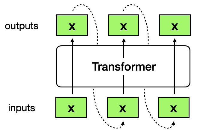
Figure 1: "Fixed points" of a Transformer preserve their values when passed through the Transformer.
Reduction to single-element sequence. Obviously, to get $[x, x, …, x] = T([x, x, …, x])$, we must at least have $[x] = T([x])$. We additionally make the observation that, for modern decoder-only LLMs using RoPE for positional encoding, as long as we find an $x$ such that $[x] = T([x])$, we have $[x, x, …, x] = T([x, x, …, x])$ for arbitrary sequence length $n$. In constrast, the original Transformers that add positional encodings as part of the input embeddings do not have this nice property.
Proof. First, consider the original Transformers (Figure 2, left). At each position, a different positional embedding vector is added element-wise to the input token embedding. Even if we found an $x$ such that if we input it at position 0, $T([x + p_0]) = [x]$, at the next position we will be transforming $[x + p_1]$ (and due to the self-attention mechanism, we will be jointly transforming $[x + p_0, x + p_1]$), and the Transformer may produce a different output $x’ \neq x$. Thus $x$ is not an FP over arbitrary sequence length.
Now consider Transformers with RoPE (Figure 2, right). We will show that the hidden states in the same layer are identical across all positions. And for that it’d suffice to show that as long as the input hidden states to a layer are identical across all positions, the output hidden states of that layer would also be identical across all positions. This is trivial for non-attention operations (e.g. FFN, LayerNorm/RMSNorm, residual connection). For self-attention blocks, RoPE is applied to transform the $Q$ and $K$ vectors in a position-dependent manner, but the $V$ vectors are identical across all positions, i.e., $v_0 = v_1 = … = v_n$ (because the input hidden states to this self-attention block are identical acorss all positions). Therefore, no matter how the attention pattern looks like, the output hidden state of this self-attention block at position $i$,
\[o_i = \sum_{j}{a_j v_j} = \sum_{j}{a_j v_0} = v_0\]is a constant and thus identical across all positions. (I omitted the out linear transformation for simplicity.) Now we have shown that the hidden states in the same layer are identical across all positions, the final outputs (which is some transformation the hidden states of the final layer) are identical across all positions, and thus all equal to $x$. This completes the proof.
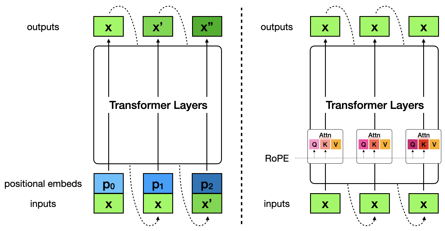 Figure 2. Left: The original Transformer with positional encodings as part of the input; $[x] = T([x])$ does not guarantee $[x, x, …, x] = T([x, x, …, x])$. Right: Modern Transformers with RoPE; $[x] = T([x])$ implies $[x, x, …, x] = T([x, x, …, x])$ for arbitrary sequence length.
Are these FPs discrete tokens or continuous vectors? You may have noticed that, so far I haven’t really said what these $x$’s are. This is where we branch and consider two possibilities: discrete tokens and continuous vectors. I will discuss them in the next two sections, respectively.
Fixed points among discrete tokens
Typically, when we use Transformers, we decode discrete tokens one-by-one. Finding discrete token FPs is interesting because it’s related to the repetition degeneration of LLMs: If you give a Transformer such a FP token $x$, it would keep decoding $x$ indefinitely.
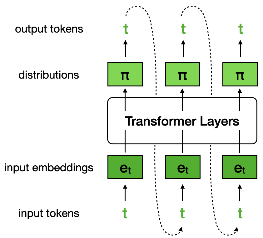
Discrete token FPs. If a Transformer receives token $t$ and outputs token $t$ (under greedy decoding), it will keep decoding token $t$ indefinitely.
There’s one nuance: Transformers output a distribution over the vocabulary – a continuous vector that is in a difference space than the input discrete token. One apparent way to resolve this is to assume we’re using greedy decoding: taking the argmax token from the output distribution. While there are other decoding algorithms, they are stochastic and thus not suitable for defining FPs.
The algorithm for finding such FP tokens is simple: We enumerate all tokens in the vocabulary, and for each token $x$, input it to the Transformer and check if $x$ has the biggest probability mass in the output distribution. Code sketch:
fps = []
with torch.no_grad():
    for x in range(tokenizer.vocab_size):
        logits = model(input_ids=torch.tensor([[x]], dtype=torch.long)).logits[0, -1, :] # (V)
        if logits.argmax().item() == x:
            fps.append(x)
Ensuring determinism in Transformers.
Some Transformers have dropout layers, which give non-deterministic results in training mode.
To ensure determinism, I set the models in eval mode (model.eval()).
I tested some open models up to 14B in the following three families: OLMo 2, Qwen 3, and Gemma 3 (both their base version and instruct version). Below is the number of discrete token FPs of each model:
| Model | Base | Inst |
|---|---|---|
| olmo2-1b | 54 | 25 |
| olmo2-7b | 101 | 15 |
| olmo2-13b | 95 | 36 |
| qwen3-0.6b | 160 | 3 |
| qwen3-1.7b | 925 | 10 |
| qwen3-4b | 651 | 13 |
| qwen3-8b | 802 | 20 |
| qwen3-14b | 866 | 8 |
| gemma3-270m | 111828 | 60086 |
| gemma3-1b | 217240 | 118373 |
A few observations:
- All models tested have discrete token FPs. Base models have more FPs than their corresponding instruct models. (Possibly related: base models tend to degenerate and repeat more than instruct models.)
- Bigger models tend to have more FPs. (Quite counter-intuitive!)
- Gemma 3 1B has way more FPs than similar-sized OLMo 2 and Qwen 3 counterparts. In fact, the majority of tokens in Gemma3-1B-Base’s vocabulary ($V = 262k$) are FPs!
Looking a bit closer into these FPs, we see that the output probability assigned to the FP tokens can vary a lot. It can be very close to 1.0 (a spiky distribution), very close to 0.0 (a nearly-uniform distribution), or something in the middle. For example, below are the top-3 and bottom-3 FP tokens of Qwen3-8B-Instruct:
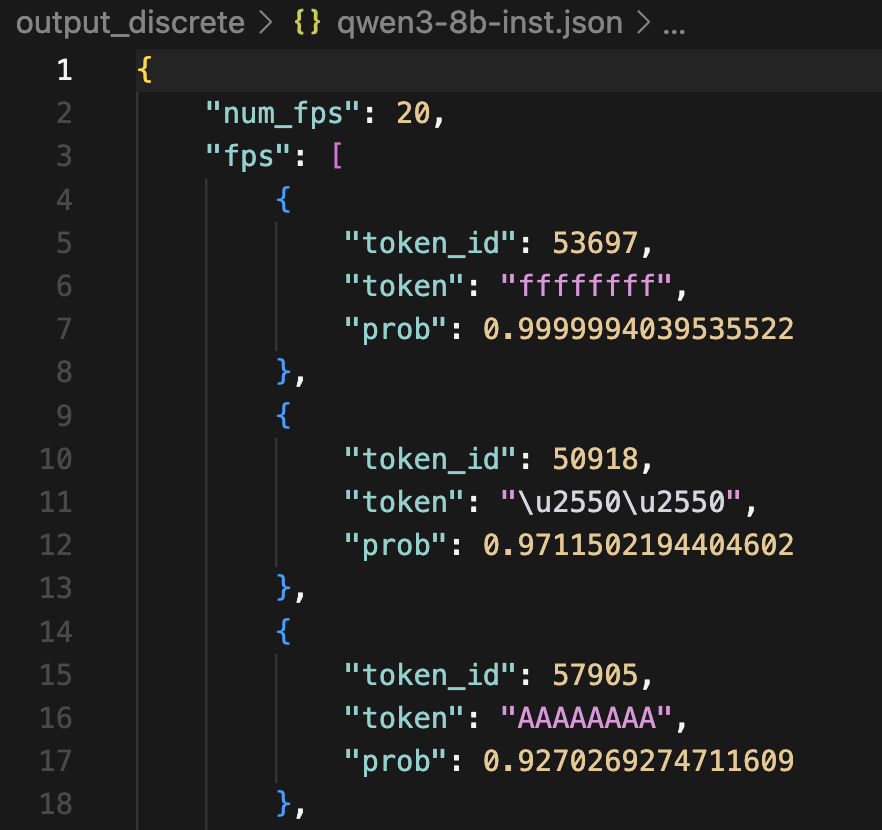
Top-3 FP tokens
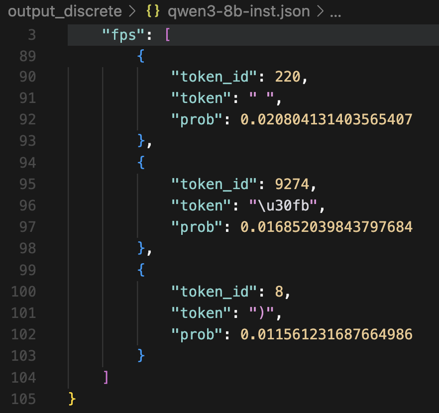
Bottom-3 FP tokens
Many FP tokens make intuitive sense.
Tokens like ????, 666, hhh, blah, and \n \n – you’d expect them to appear repetitively in many training documents.
One nice thing with fully-open LLMs like OLMo 2 is that we can inspect the training data (with infini-gram search) to verify this.
For example, blah is an FP token of OLMo2-13B-Base, and we can find 66k occurrences of its 10-repetition:

For some other tokens, it’s not obvious why they became FPs, and searching in data can shed some light.
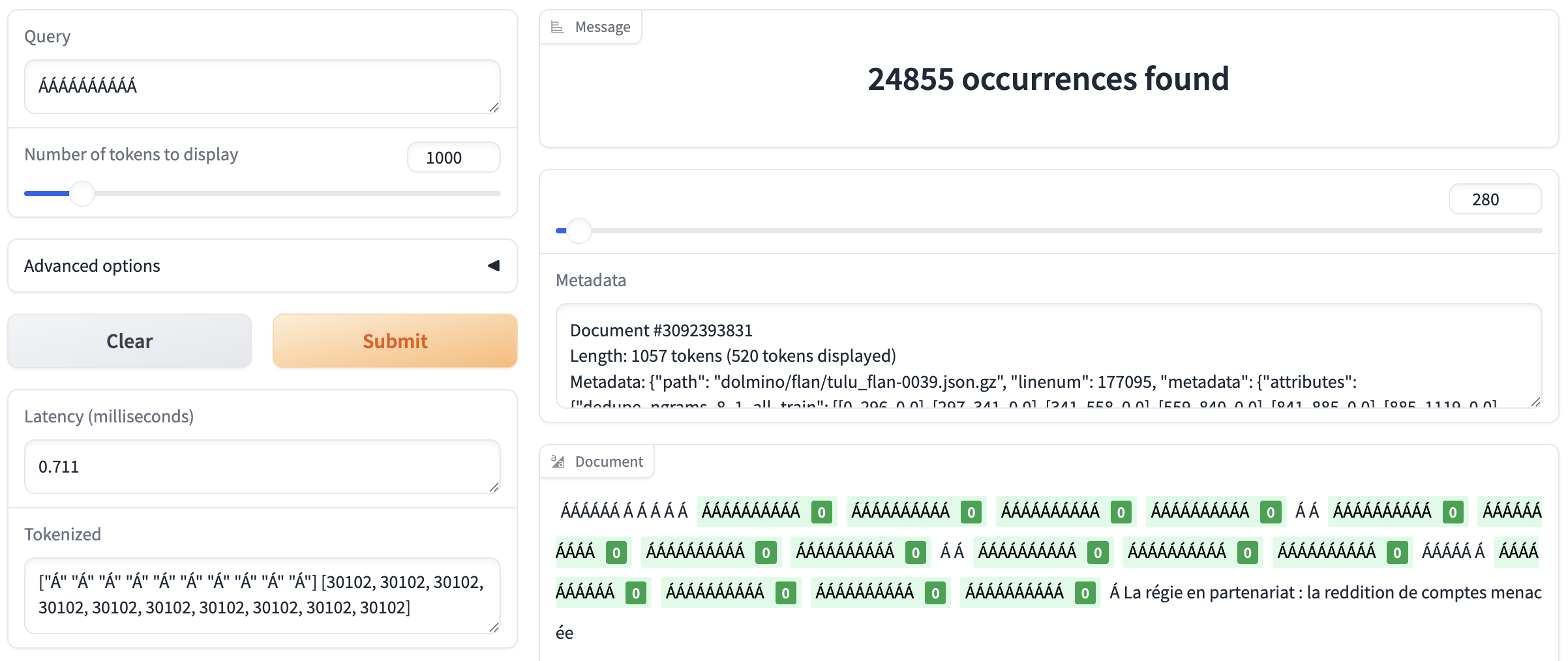
The top-1 FP token of OLMo2-13B-Instruct is \u00c1 (which is latin letter Á with an acute accent).
String ÁÁÁÁÁÁÁÁÁÁ appears 25k times in this model’s full training data (mostly from the Flan set used in mid-training, for some mysterious reasons):
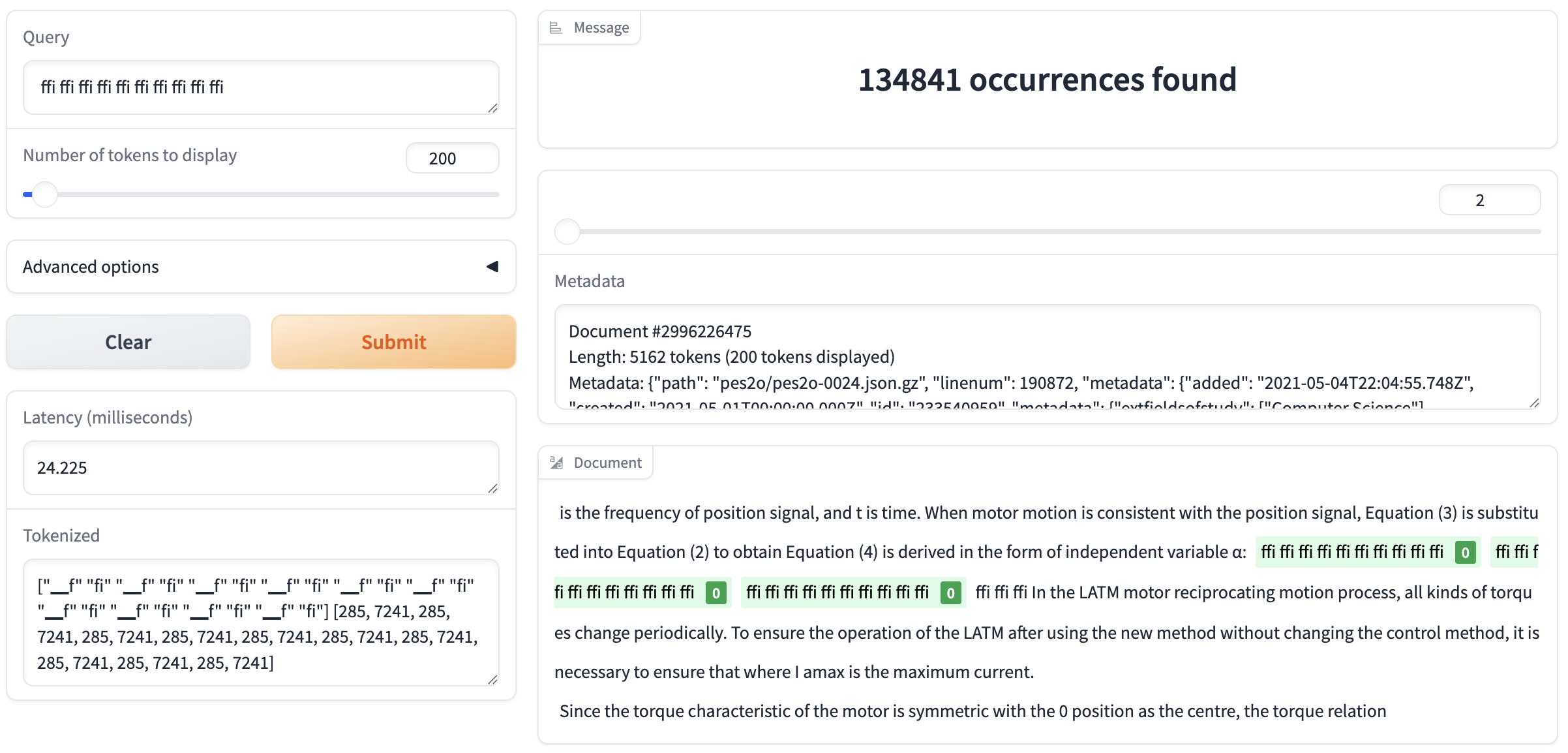
Another top FP token among OLMo 2 models is ffi, which appears to be due to incorrect parsing of equations in the pes2o dataset (Semantic Scholar papers) used in pre-training the OLMo 2 family:
I also noticed that LLMs in the same model family share many common FP tokens.
As an example, \u00c1 is an FP token for all OLMo 2 models I tested.
This corroborates with my intuition that FPs are closely tied to the training data.
FP tokens seem promising to be used to identify problematic training data, and to infer some training data of open-weight LLMs.
Fixed points in the embedding space
Now we move on to consider continuous vector FPs. Transformers embed the input discrete tokens into vectors $x \in \mathbb{R}^D$, which are subsequently sent into the Transformer layers. We can try to find FPs in this embedding space $\mathbb{R}^D$.
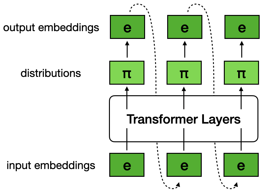
Continuous FPs in the embedding space. The FPs are not necessarily the exact embedding of any particular token, but is a weighted mixture of the embeddings of many tokens in the vocabulary.
The Transformer model outputs a distribution $y \in \Delta^V$ over the vocabulary. Now the good news is, we no longer need to assume greedy decoding, which can look like a compromise. But we still need to convert this distribution into the embedding space. One apparent way is to take a weighted mixture of the token embeddings according to this distribution. Mathematically, this would be simply multiplying this distribution vector $y$ with the embedding matrix $E$: $y E \in \mathbb{R}^D$. We can think of the transformation function $T$ associated with the Transformer model as $T(x) := y E$. The continuous FPs we’re looking for should satisfy $x = T(x) = y E$.
Below I will discuss two ways for finding FPs in this embedding space: (1) fixed-point iteration, and (2) gradient descent.
Fixed-point iteration
Fixed-point iteration is a simple method for finding the FP of a function $f$ with the same domain and codomain. Starting from an arbitrary point $x_0$, it iteratively computes $x_{n+1} = f(x_n)$ until the sequence converges. The final obtained $x_N$ ($N$ as determined by some stopping criteria) is an FP of $f$.
A bit of theory. Under a few conditions, this method guarantees convergence to an FP. (See Banach fixed-point theorem.) The conditions are: (1) $f$ is a continuous function, and (2) $f$ is a contraction mapping, roughly meaning any perturbation on the input cannot shift the output by a distance larger than the magnitude of the perturbation itself. In addition, under these conditions, the FP of function $f$ is unique.
These two conditions are generally not met by the Transformer function $T(x)$. For (1), there will always be numerical errors in floating-point operations. For (2), we have no guarantee that an arbitrary pretrained Transformer represents a contraction mapping. In fact, as I will show later, we can often find multiple vector FPs for a given LLM, implying that at least one condition is broken.
That said, I still gave it a shot. Here’s a sketch of the code:
x = torch.nn.Parameter(torch.randn(D, dtype=torch.float32) * model.config.initializer_range) # (D)
while loss > EPS:
    with torch.no_grad():
        logits = model(inputs_embeds=x[None, None, :]).logits[0, -1, :] # (V)
        probs = F.softmax(logits) # (V)
        y = probs @ embed_matrix # (D)
        loss = torch.norm(y - x)
        x = y
Experiment setup. I keep iterating until the L2 distance between the input and output falls below a threshold $\varepsilon$, and in practice I use $\varepsilon = 10^{-6}$. Since the outcome depends on the random initial $x$, I run each LLM 10 times with different seeds and aggregate results. In some runs, ${x_n}$ doesn’t converge, and I removed those results. If a found FP is within an L2 distance of $10^{-4}$ from another FP, I say that these two FPs are identical and only keep one.
I tested on the same set of open-weight LLMs as in the last section. Below is the number of continuous vector FPs found by fixed-point iteration for each model:
| Model | Base | Inst |
|---|---|---|
| olmo2-1b | 0 | 2 |
| olmo2-7b | 1 | 1 |
| olmo2-13b | 1 | 1 |
| qwen3-0.6b | 1 | 1 |
| qwen3-1.7b | 1 | 1 |
| qwen3-4b | 1 | 1 |
| qwen3-8b | 2 | 2 |
| qwen3-14b | 1 | 0 |
| gemma3-270m | 1 | 1 |
| gemma3-1b | 0 | 0 |
A few observations:
- For most models, fixed-point iteration can find either 1 or 2 FP vectors. In case of a few models, the method fails to find any. Note that this may not be all the vector FPs: some might have a small range of initialization $x_0$ that can converge to them, and we might be missing them due to not having more trials. Doing 10 trials should have covered the most “popular” FP vectors.
- The number of FP vectors found is magnitudes fewer than FP tokens. Of course, fixed-point iteration may be missing some FP vectors, but I suspect that the definition of FP becoming more strict (with the removal of greedy decoding) also contributed to this.
- When fixed-point iteration converges, it typically converges within a few dozen steps. I ran all experiments up to 10,000 steps, and found that if it doesn’t converge within 200 steps, it won’t converge even given more steps.
Token compositions of FP vectors.
An FP vector can be viewed as a weighted mixture of tokens in the vocabulary.
To get a more intuitive understanding of these FP vectors, we can look at the top-contributing tokens in this mixture.
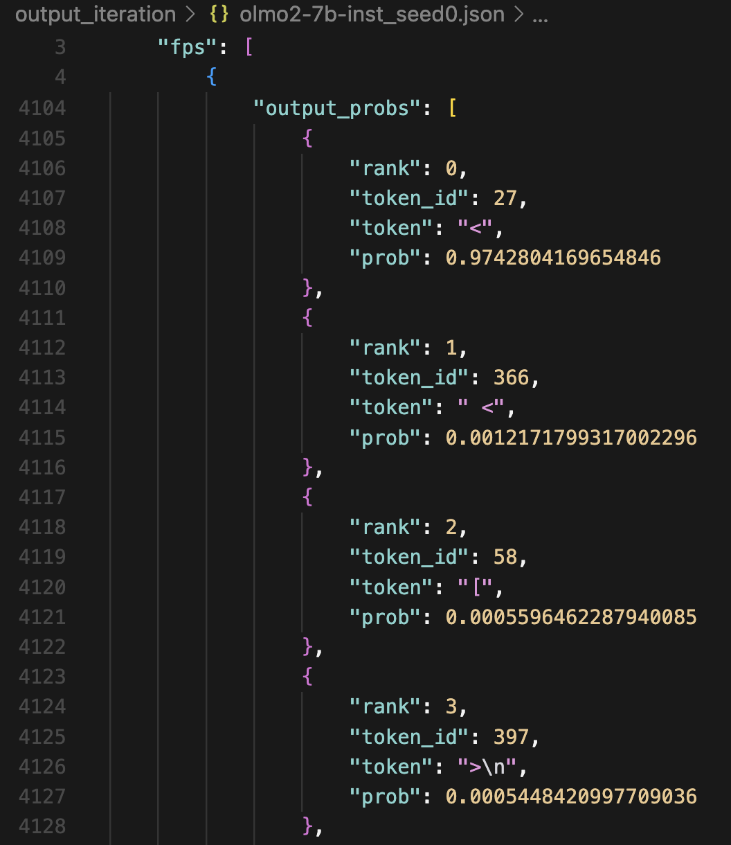
For example, the FP vector of OLMo2-7B-Instruct is 97% from the embedding of token < and 3% contributed by other tokens (and in fact, < is a discrete token FP of this model).
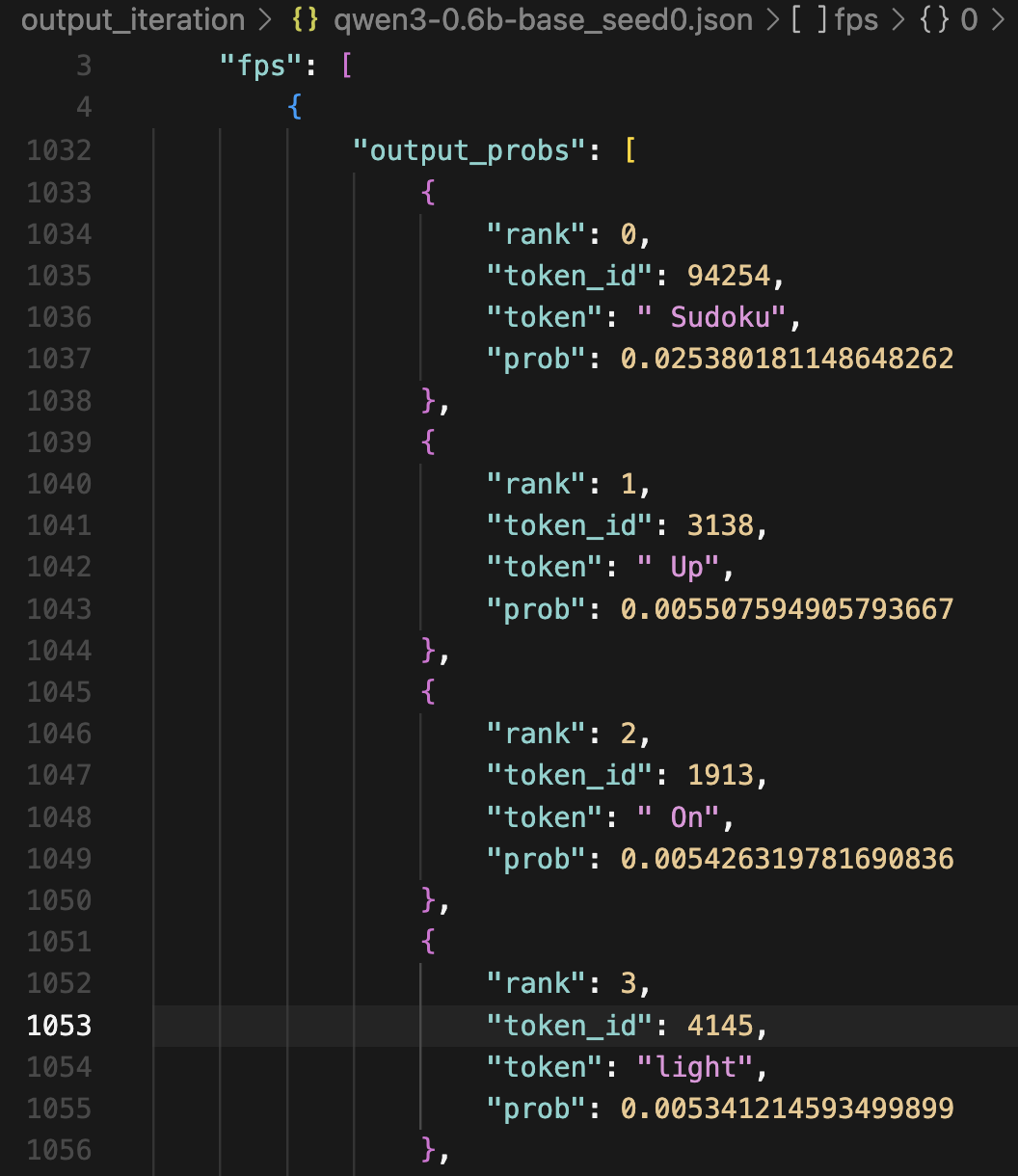
Meanwhile, some other FP vectors have quite “flat” mixtures.
The top token ( Sudoku) only contributed 2.5% to the FP vector of Qwen3-0.6B-Base.
Numerical errors & “unstable” FP vectors. Due to floating point errors, the FP vectors we found are not strict FPs. Following our stopping criteria, the input and output vectors may have an L2 distance (i.e., an error) up to $10^{-6}$. Running more iteration steps could not further reduce this error down to 0. This creates a problem with the reduction we made at the beginning of this post – from solving $T([x, x, … x]) = [x, x, …, x]$ to solving $T([x]) = [x]$. With autoregressive decoding, the FP vectors might diverge due to these numerical errors.
In practice, I observed two types of FP vectors – “stable” ones where the error is bounded by a small value during autoregressive decoding, and “unstable” ones where the error blows up.
Most of the FP vectors found above are stable, with one exception from Qwen3-1.7B-Instruct.
Below are examples of stable and unstable FPs.
In each example, the rollout_dist_by_l indicates for each decoding sequence length $l$, the L2 distance between the final output vector at the last position and the initially-found FP vector; rollout_dist_max is the maximum of such distances over $l = 1 … 100$.
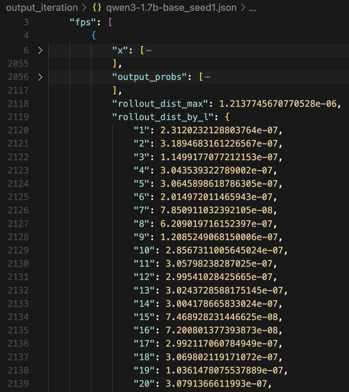
The FP vector found for Qwen3-1.7B-Base is a stable FP. The max error over decoding 100 tokens is in the order of $10^{-6}$.
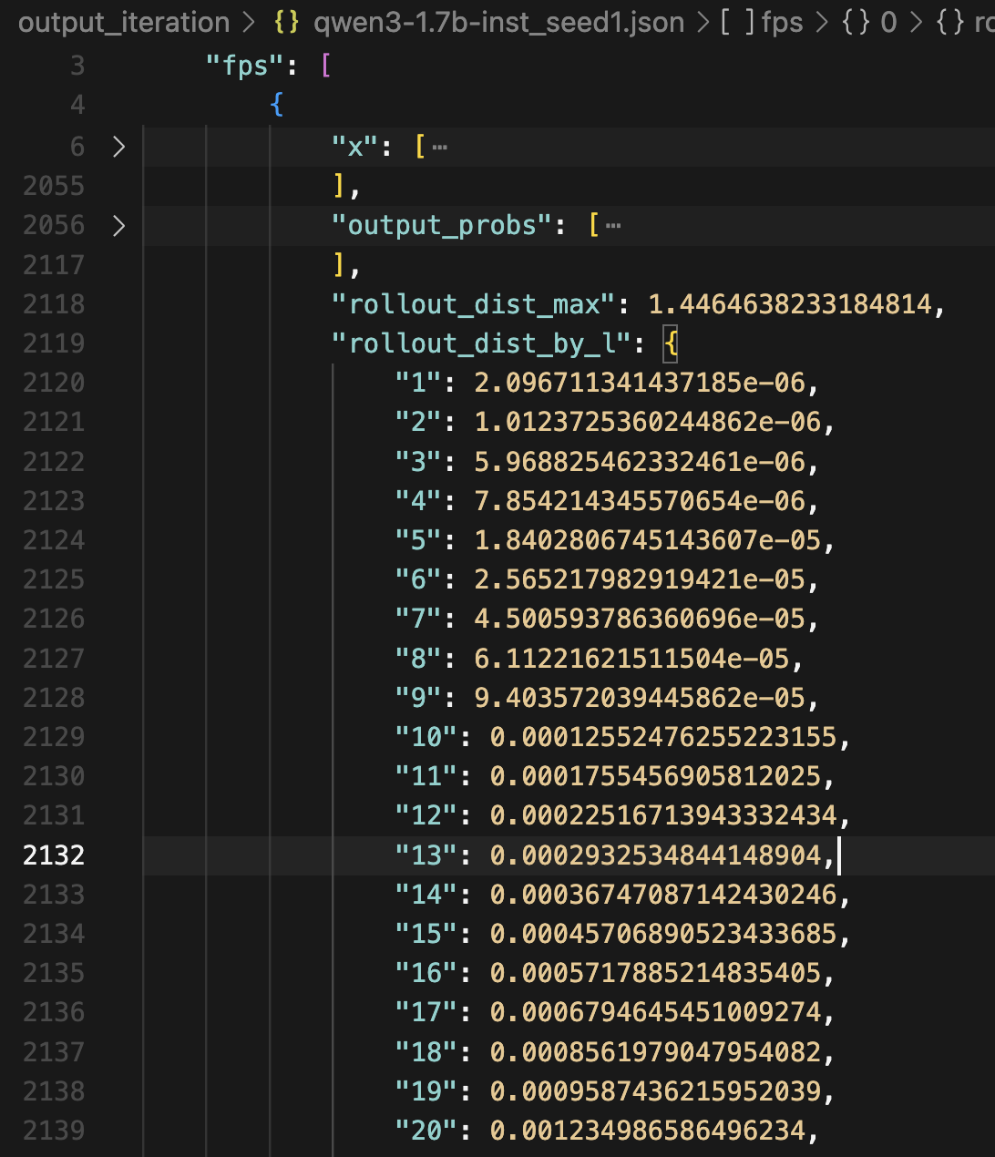
The FP vector found for Qwen3-1.7B-Instruct is an unstable FP. Although the error on decoding the first token is low ($2.09 \times 10^{-6}$), the error compounded over autoregressive decoding, and the max error over decoding 100 tokens is above 1.0.
Gradient descent
Gradient descent is a common way to optimize continuous values towards a target. In our case of finding FPs, our target is to make the output $T(x)$ match the input $x$. We can thus define a loss to optimize for, e.g., an L2 distance loss: \(L_x = || x - T(x) ||_2\) and use gradient descent to optimize this loss. Contrary to typically LLM training where the Transformer parameters $\theta$ are optimized, here we fix $\theta$ and optimize the input vector $x$.
Gradient descent as a generalization of fixed-point iteration. Consider a scenario where we use a squared L2 loss and do not backprop the gradient through $T(x)$, i.e., $L_x = \Big( x - \text{detach} \big( T(x) \big) \Big) ^2$. Then we have gradient $\partial{L} / \partial{x} = 2 (x - T(x)) $. If we use learning rate $\eta = 0.5$, then the gradient update step would reduce to $x \leftarrow x - \eta \cdot \partial{L} / \partial{x} = x - 0.5 \cdot 2 (x - T(x)) = T(x)$, which is identical to fixed-point iteration.
In practice, I found detaching $T(x)$ gives better and faster convergence.
I use L2 distance loss.
I use AdamW optimizer with initial LR $10^{-2}$ and a ReduceLROnPlateau scheduler.
For each LLM, I run 10 times with different random initialization of $x$.
Here’s a sketch of the code:
x = torch.nn.Parameter(torch.randn(D, dtype=torch.float32) * model.config.initializer_range) # (D)
lr = 1e-2
while lr > 1e-9:
    with torch.no_grad():
        logits = model(inputs_embeds=x[None, None, :]).logits[0, -1, :] # (V)
        probs = F.softmax(logits) # (V)
        y = probs @ embed_matrix # (D)
    loss = torch.norm(y - x)
    loss.backward()
    optimizer.step()
    lr = scheduler.step()
Below is the number of continuous vector FPs found by fixed-point iteration for each model: (the number in parentheses is difference with the number of FP vectors found in fixed-point iteration)
| Model | Base | Inst |
|---|---|---|
| olmo2-1b | 3 (+3) | 5 (+3) |
| olmo2-7b | 1 | 1 |
| olmo2-13b | 1 | 1 |
| qwen3-0.6b | 1 | 1 |
| qwen3-1.7b | 2 (+1) | 1 |
| qwen3-4b | 2 (+1) | 1 |
| qwen3-8b | 2 | 5 (+3) |
| qwen3-14b | 2 (+1) | 3 (+3) |
| gemma3-270m | 1 | 1 |
| gemma3-1b | 0 | 1 (+1) |
A few observations:
- Gradient descent finds more vector FPs than fixed-point iteration. This corroborates my previous note that fixed-point iteration may not find all FPs with limited trials.
- That said, the vector FPs found by gradient descent may not be complete, either. While most vector FPs found by fixed-point descent are also found by gradient descent, there are a few exceptions.
- The additional FP vectors found by gradient descent are a mixture of stable and unstable FPs.
You ask BF16?
I all experiments, I use FP32 for model weights and input tensors. I tried using BF16 for them, but the results are not good. With fixed-point iteration, BF16 usually does not converge to a point with low error. With gradient descent, the loss (i.e. error) does not reach a low enough point before diverging. Both indicates that finding FPs needs higher floating point precision beyond BF16.
Closing thoughts
This is one of my pet projects. I had the initial idea more than 4 years ago, right after I started my PhD. Back then, I did some experiments but it didn’t work because LLMs were largely on additive position encodings. Later, RoPE was proposed and got widely adopted in mordern LLMs, so I found time to revisit this idea. I did this purely for fun and intellectual curiosity, and it happens to bring some unexpected findings.
If this inspires some ideas in you, please feel free to reach out and I’m happy to chat!
Code is available here.