Bottom-Fishing in Market Crash
Every couple of years, there is a market correction, or even a market crash. However, historical data tells us that the market will always come back, so we want to buy at cheap price during such time, in hope to make a large return when the market comes back. How should we do this given no one knows where the “real” bottom is in advance? We need a strategy.
You can choose any market metric to track: S&P 500, NASDAQ, or the price of an ETF. For simplicity, we assume that the peak metric observed before market crash is \$1. The metric will keep falling until it hits \$$M$ ($M$ is unknown to us), after which it will come back. Based on the exponential thinking principle, we assume that $m \sim \text{exp}(\lambda)$, where $m = -\ln{M}$ and $\lambda$ is a parameter based on the nature of the market. We evaluate our return when the metric comes back to \$1.
Here’s our strategy, in formal language. We choose parameters $p > 1, 0 < s < 1$. Whenever the metric is divided by $p$, we buy a certain dollar amount of the underlying asset at the market price. The dollar amount bought each time is $s$ times the amount bought in the previous time.
| When the metric falls to … | Buy … dollars | Buy … shares |
|---|---|---|
| $p^{-1}$ | $s$ | $s p$ |
| $p^{-2}$ | $s^2$ | $(s p)^2$ |
| $p^{-3}$ | $s^3$ | $(s p)^3$ |
| … | … | … |
| $p^{-n}$ | $s^n$ | $(s p)^n$ |
| … | … | … |
Apparently when the metric comes back to \$1, the total value of our asset is equal to the total number of shares we bought. Our return is the total value divided by the total contribution. If the price dips at $M \in (p^{-(n+1)}, p^{-n}]$, our return will be
\[R_n = \frac{sp + (sp)^2 + ... + (sp)^n}{s + s^2 + ... + s^n} = \frac{(1-s) p}{1-sp} \frac{1 - (sp)^n}{1 - s^n}\]with probability $P_n = p^{-n \lambda} (1 - p^{-\lambda})$. We define $R_0 = 0$. The expected return is $\mathbb{E}[R] = \sum_{n=0}^{\infty}{P_n R_n}$. We assume that $\lambda > 1$, so that the expected return always converges. This objective cannot be optimized analytically, so we take a look at the plot: (with $\lambda = 1.5$)
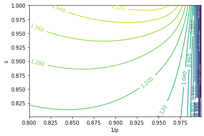
If we restrict to $s = 1$, we will find that the optimal $p = 0.940$, which does not degenerate. This means a good strategy is to buy a constant amount every time the metric falls by 6%.
How do we choose the value of $\lambda$? Let’s take a look at historical data. We consider S&P market corrections of 20% or more since 2000, collect the value $m$ of each correction, and make a MLE estimate of $\lambda$. This gives us $\hat{\lambda} = 1.555$. When we plug this into the expected return plot, we find that the optimal $p = 0.945$.